Controlling Dynamic Components Models

 

For more information on Dynamic Component Models see Pasdirtz, 2007.

Error Correcting Controllers in the World-System

 

Error Correcting Controllers (ECC) are used in Control Theory to generate positive and negative feedback loops to control systems. In economics and sociology, ECCs can be generalized to describe the behavior of macro-economic and macro-social systems starting with Leibenstein's Malthusian Model:

• Malthusian Controller (Q-N) Negative feedback will result when population growth exceeds economic growth.
• Stock Adjustment (Q-K)
• Liberal Market Controller (Q-P) 
• Marxist Controller (Q-L) or (Q-wL) 
• Labor Surplus Controller (Q-LA) 
• Keynesian Controller (Q-G) 
• Environmental Controller (Q-T) 
• Mercantilism Controller (Q-X)
• Modernization Controller (N-V)
• World Price Controller (XR-X)
• Monetarism Controller  (Q-M)
• Fascism Controller (Q-War)
• Globalization Controller (WS-QP)
• Malthusian Trade Controller (N-X)
• Liberal Trade Controller (Q-X)
• Labor Surplus Controller (X-L)
• Class Struggle Controller (L-U)
• Urban Trade Controller (X-U)
• World-System Controller (WS-X)
• Ricardian Trade Controller (X-XWS)

In specific countries during specific historical periods, combinations of controllers are likely to be used. The used of an ECC or multiple ECCs does not imply that the systems is under stable control. For more discussion, see Growth and Control in the World-System. You can run the US_M model code and experiment with the model (here).

Growth and Control in the World-System

 

Taking a systems perspective on societal development involves (1) finding measurable variables of interest for the system and (2) categorizing them using the graphic above. Input variables are external to the system, for example the economic growth of another country or of the World System. Output variables are those under control of the system. The Environment captures the qualitative factors that might influence the performance of the system during a specific historical period. Feedback Control involves (1) the dynamic interactions of the state variables over time and (2) a feedback control loop (for example a PID Controller) imposed on a system to produce desired outputs.

Needless to say, for a macro-economic system, input and output variables could involve an infinite number of measurements. State Variables are the independent set of variables that explain the time path of the system outputs in response to inputs. In Dynamic Component Models, approximate state variables are constructed using Principle Components Analysis. Weightings and signs of indicator variables are used to construct the Measurement Matrix which converts state variables to output variables.

The measurement matrix for the US_M Model (1900-2000) shows a number of controllers. Each row of the matrix is a state variable. The first state variable describes Overall Balanced Growth. The second state variable, US2=(0.663X - 0.555N) describes a Malthusian Export Controller. The third state variable describes a combination of controllers: Malthusian = (0.484 Q - 0.421 N),  Export Prices = (0.33 XREAL - 0.538 X) and Employment = (0.3458 HOURS - 0.268 L). Together, these three state variables explain 0.999% of the variation in the growth indicators.

The time plots for the US1, US2 and US3 state variables are presented above. US1 is the growth component that shows an exponential path across the Long 20th Century. US2 (dashed red line) the Malthusian Export Controller turns negative in the period after 1960. And, US3, the complex Malthusian, Export-Price and Employment controller stays close to the zero point throughout the period.

The three short-cycle minor controllers, US4= (0.650 Q- 0.504 L), (US5=(0.7362 HOURS- 0.490 L)) and (US6=another complex controller), show cyclical paths with decade-long periods.

World-System (1300-1450): The German Economy

 

One of the most important points to understand about Germany is that until 1871 Unification, Germany was a collection states and part of the Holy Roman Empire. Cities were connected by crude trading routes and the size of the cities was limited by the difficulties of long term trade. Urbanization (DE3=(U-N) above) was a strong limiting factor in economic development for the period prior to 1450 (see the graphic above). Growth did not begin accelerating until 1409. And the period prior to 1409 was a long-developing Malthusian Crisis (U-N) that limited expansion.

The period from 1300-1400 is sometimes called the Crisis of the Middle Ages: demographic collapse, political instability and religious upheaval. The Great Famine of 1315–1317 and the Black Death of 1347–1351 potentially reduced the European population by half or more as the Medieval Warm Period came to a close and the first century of the Little Ice Age began and unity of the Catholic Church was threatened by the Western Schism. In Germany between 1336 and 1525 there was widespread and militant peasant unrest.   Both the Urbanization ECC and the Malthusian ECC worked together to limit growth up to 1409. 

Economically, the period after 1300 in the graphic above was dominated by the  Hanseatic League which declined after 1450. Hanseatic trade involved both maritime, in-land waterway and overland trade.

State Space Models for the period (1300-1450) can be found here.  A discussion of the period after 1450 can be found here.

Notes

The measurement matrix for the state space model is presented above. DE1=(Growth), DE2=(Q-N-U) and DE3=(U-N), that is Growth, the Urban-Malthusian Controller and the Urbanization Controller (A discussion of Error Correcting Controllers, ECCs, can be found here).

World-System (1450-1640): The German Economy

 

The expansion of the German Economy after 1450 (a discussion of the period before 1450 can be found here)  was brought to an end by the Urbanization Controller (Q-U) which peaked about 1550 which was also associated with a mild Malthusian crisis (Q-N). Eventually, growth reached a plateau after 1600.

During the early part of the Long Sixteenth Century (1450-1650), the Great Bullion Famine also limited economic growth. Precious metals were necessary to conduct overland and maritime commerce and the European mines were being played out. The voyages of Columbus were motivated by the search for gold necessary to mint coin.

Notes

The measurement matrix for the DEL16 state space model is presented above showing the weightings for the Urbanization (0.634 Q - 0.768 U) and the Malthusian (0.524 Q - 0.7821 N) Error Correcting Controllers (ECCs).

The system matrix for the DEL16 state space model is presented above. The model is unstable (dominant eigenvalue greater than 1.0). The model can be stabilized by reducing the coefficient for the Urbanization ECC (F[2,2] = 1.017812347) or you can turn the Urbanization and the Malthusian ECCs into random walks by setting (F[2,2] = F[3,3] = 1.0).

The result of setting the ECCs to random walks is to create a cyclical system (see the forecast above). What is interesting is that this cyclical system, without German Unification in 1871, enters the Twentieth Century, right before WWI, on a downward cycle. Germany would have been unable to wage war without Unification (see Pasdirtz, 1981).

State Space models for the period (1450-1640) can be found here.

Boiler Plate

State Space Model Estimation

The Measurement Matrix for the state space models was constructed using Principal Components Analysis with standardized data from the World Development Indicators. The statistical analysis was conducted in an extension of the dse package. The package is currently supported by an online portal (here) and can be downloaded, with the R-programming language, for any personal computer here. Code for the state space Dynamic Component models (DCMs) is available on my Google drive (here) and referenced in each post.

Atlanta Fed Economy Now

My approach to forecasting is similar to the EconomyNow model used by the Atlanta Federal Reserve. Since the new Republican Administration is signaling that they would like to eliminate the Federal Reserve, the app might well not be available in the future.

While the app is still available, there have been some interesting developments. In earlier forecasts, the Atlanta Fed was showing GDP growth predictions outside the Blue Chip Consensus. Right now, after unorthodox economic policies from the Trump II Administration, the EconomyNow model is predicting a drastic drop in GDP (the Financial Forecast Center is only predicting a slight drop here).

Climate Change

Another comparison for what I have presented above are the IPCC Emission Scenarios. These scenarios are for the World System. Needless to say, (1) the new Right-Wing Republican administration plans on withdrawing the US from all attempts to study or ameliorate Climate Change and (2) the IPCC does not produce any RW modes for the World System (but seem my forecasts here).

World System

The longest running set of data we have for the World-System is the Maddison Project based on the work of Angus Maddison (more information is available here). Data on production (Q) and population (N) for most countries and regions runs from years 0-2000. More data becomes available as we near the year 2000. 

Available data were entered in a spreadsheet (see Population above, double click to enlarge). Missing data were interpolated with nonlinear spline smoothing using the R programming Language.

In cases where initial values were not available (see GDP above), the E-M Algorithm was used to estimate initial conditions.

From the graph of GDP above (W_Q) for the World System, it can be seen that economic growth from the year 0-1500 was basically flat. The period of British Capitalism (after 1500) had a small plateau of growth. Takeoff does not happen until the Nineteenth Century.

From a system's perspective, the only model that can be tested for the entire period is Kenneth Boulding's Malthusian Systems Model [Q,N] = f[Q,N].

When developed as a State Space model (measurement matrix above) there are two components: W1=Growth and W2=(Q-N), the Malthusian Controller. When more data is available, the Malthusian Controller can be generalized to other SocioEconomic theories.

What the Malthusian Controller shows (plotted as Q-N above) is that a long-developing Malthusian Crisis (Q<N) started in the Late Middle Ages and accelerated through the period of British Capitalism (Dark Satanic Mills) and was reversed spectacularly during the Nineteenth Century.  Takeoff in response to a deepening Malthusian Crisis would not be an unreasonable way to view Modern Economic Growth.

Error Correcting Controllers (ECC)

In another post (here), I presented Leibenstein's Malthusian Error Correcting Controller (ECC). It can be generalized to the dominant ECCs in most theoretical economic models (above). These controllers can be further generalized. For example, (X-U) and (L-U) can be generalized to (N-U), a more general Urbanization Controller which describes market expansion for economic growth. In countries and periods with limited data, (N-U) might subsume all these processes. ECCs describe important feedback processes in SocioTechnical System that are typically not recognized as such in academic literature.

Kaya Identity

The basic theoretical model underlying all the World-System models I crate is the Kaya Identity. There are a number of advantages to starting theoretical development with the Kaya Identity: (1) An "identity" is true by definition Adding other variables to the model ensure that theory construction is on a solid footing. (2) The Kaya Identity is also used as the foundation for the IPCC Emissions Scenarios allowing a linkage between World-Systems Theory and the work of the IPCC.

World Development Indicators (WDI)

After WWII, extensive data sets on all countries in the World-System became available from the World Bank (here). The indicators above where chose to construct the state space for each WDI-based model. Addition indicators can be added for specific forecasts and analyses.

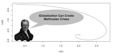
World-System (1950-2010): The Ukrainian Economy

 

Notes

You can run the full UAL20 BAU model here and explore the other Error Correcting Controllers (ECC) which have complicated Malthusian elements.

Black Box, Isomorphic Cybernetic Systems

 

Cybernetics played an important role in the development and control of mechanical-electric systems but did not gain traction in the Social Sciences.

Political systems Theory

Notes

Ashby, Ross (1956) An Introduction fo Cybernetics, (pdf file).

Lange, Oskar (1970) Introduction to Economic Cybernetics (pdf file).

Steinbrenner, John (1974) Cybernetic Theory of Decision Making: New Dimensions in Political Analysis.

Easton, David (1900) The Political System